معرفی نرم افزار هوشمند نوین

نمایندگی رسمی نرم افزار حسابداری هوشمند نوین در استان اردبیل

الگوریتم PSO

الگوریتم بهینه سازی ازدحام ذرات (Particle Swarm Optimization) یا به اختصار PSO یکی از مهم ترین الگوریتم های بهینه سازی هوشمند است که در حوزه هوش ازدحامی (Swarm Intelligence) جای می گیرد. این الگوریتم توسط جیمز کندی (James Kennedy) و راسل سی ابرهارت در سال ۱۹۹۵ معرفی گردید و با الهام از رفتار اجتماعی حیواناتی چون ماهی ها و پرندگان که در گروه هایی کوچک و بزرگ کنار هم زندگی می کنند، طراحی شده است. در الگوریتم PSO اعضای جمعیت جواب ها به صورت مستقیم با هم ارتباط دارند و از طریق تبادل اطلاعات با یکدیگر و یادآوری خاطرات خوب گذشته به حل مساله می پردازند. الگوریتم PSO برای انواع مسائل پیوسته و گسسته مناسب است و پاسخ های بسیار مناسبی برای مسائل بهینه سازی مختلف داده است.

الگوریتم زنبورها Bees Algorithm

یکی از نسخه های معروف از دسته الگوریتم های مبتنی بر زنبورهای عسل مورد بررسی قرار گرفته است، که به نام الگوریتم زنبورها (زنبوران) و یا Bees Algorithm (به اختصار BA) شناخته می شود.

زنبورهای عسل از جمله حشراتی هستند که در کلونی ها و مجموعه های نسبتا بزرگ در کنار یکدیگر زندگی می کنند. علاوه بر منافعی که در زمینه کشاورزی، باغداری و تولید عسل و موم از این حشره مفید کسب می شود، رفتار اجتماعی منظم این موجودات، همواره منشا الهام و مبدا مطالعات علمی قرار گرفته است. تاکنون نسخه های مختلفی از الگوریتم های بهینه سازی ارائه شده اند، که از رفتار گروهی زنبورها برگرفته شده اند.

الگوریتم مورچگان Ant Colony

بهینه سازی کلونی مورچه ها (Ant Colony Optimization) و به اختصار ACO، که در سال ۱۹۹۲ توسط مارکو دوریگو (Marco Dorigo) و در رساله دکتری ایشان مطرح شد، یکی از بارزترین نمونه ها برای روش های هوش جمعی است. این الگوریتم از روی رفتار جمعی مورچه ها الهام گرفته شده است. مورچه ها با همکاری یکدیگر کوتاه ترین مسیر را میان لانه و منابع غذایی پیدا می کنند تا بتوانند در کمترین زمان، مواد غذایی را به لانه منتقل کنند. هیچ کدام از مورچه ها به تنهایی قادر به انجام چنین کاری نیستند، اما با همکاری و پیروی از چند اصل ساده بهترین راه را پیدا می کنند. الگوریتم مورچه ها، یک مثال بارز از هوش جمعی هستند که در آن عامل هایی که قابلیت چندان بالایی ندارند، در کنار هم و با همکاری یکدیگر می توانند نتایج بسیار خوبی به دست بیاورند.

ارايه الگوريتم رقابت استعماري چندهدفه جهت بهينه سازي مساله ي برنامه ريزي

در اين مقاله، مدلي دوهدفه براي يک مساله ي برنامه ريزي توليد ادغامي چندمحصولي چند دوره اي در زنجيره تاميني شامل تعدادي تامين کننده، توليدکننده و نقطه تقاضا ارائه شده است که از يک طرف به دنبال کمينه سازي هزينه کل زنجيره تامين شامل هزينه هاي نگهداري موجودي، هزينه هاي توليد، هزينه هاي نيروي انساني، هزينه هاي جذب و از دست دادن نيروي انساني مي باشد و از طرف ديگر و به صورت همزمان با استفاده از بيشينه سازي حداقل قابليت اطمينان کارخانه هاي توليدي با در نظر گرفتن زمان هاي تحويل احتمالي، به دنبال بهبود عملکرد سيستم و برنامه توليد پاياتري است. در نهايت با توجه به اينکه مساله مذکور NP-hard مي باشد، براي حل مدل پيشنهادي از يک الگوريتم رقابت استعماري چندهدفه مبتني بر پارتو استفاده شده و به منظور بررسي عملکرد الگوريتم مذکور، الگوريتم ژنتيک مرتب سازي نامغلوب (NSGA-II) نيز بکار رفته است. نتايج حاصل از مسائل آزمايشي توليد شده، توان الگوريتم پيشنهادي را در يافتن جواب هاي پارتو نشان مي دهد.

الگوریتم PSO

Particle Swarm Optimization

Introduction

Inspired by the flocking and schooling patterns of birds and fish, Particle Swarm Optimization (PSO) was invented by Russell Eberhart and James Kennedy in 1995. Originally, these two started out developing computer software simulations of birds flocking around food sources, then later realized how well their algorithms worked on optimization problems.

Particle Swarm Optimization might sound complicated, but it's really a very simple algorithm. Over a number of iterations, a group of variables have their values adjusted closer to the member whose value is closest to the target at any given moment. Imagine a flock of birds circling over an area where they can smell a hidden source of food. The one who is closest to the food chirps the loudest and the other birds swing around in his direction. If any of the other circling birds comes closer to the target than the first, it chirps louder and the others veer over toward him. This tightening pattern continues until one of the birds happens upon the food. It's an algorithm that's simple and easy to implement.

The algorithm keeps track of three global variables:

• Target value or condition
• Global best (gBest) value indicating which particle's data is currently closest to the Target
• Stopping value indicating when the algorithm should stop if the Target isn't found

Each particle consists of:

• Data representing a possible solution
• A Velocity value indicating how much the Data can be changed
• A personal best (pBest) value indicating the closest the particle's Data has ever come to the Target

 

The particles' data could be anything. In the flocking birds example above, the data would be the X, Y, Z coordinates of each bird. The individual coordinates of each bird would try to move closer to the coordinates of the bird which is closer to the food's coordinates (gBest). If the data is a pattern or sequence, then individual pieces of the data would be manipulated until the pattern matches the target pattern.

The velocity value is calculated according to how far an individual's data is from the target. The further it is, the larger the velocity value. In the birds example, the individuals furthest from the food would make an effort to keep up with the others by flying faster toward the gBest bird. If the data is a pattern or sequence, the velocity would describe how different the pattern is from the target, and thus, how much it needs to be changed to match the target.

Each particle's pBest value only indicates the closest the data has ever come to the target since the algorithm started.

The gBest value only changes when any particle's pBest value comes closer to the target than gBest. Through each iteration of the algorithm, gBest gradually moves closer and closer to the target until one of the particles reaches the target.

It's also common to see PSO algorithms using population topologies, or "neighborhoods", which can be smaller, localized subsets of the global best value. These neighborhoods can involve two or more particles which are predetermined to act together, or subsets of the search space that particles happen into during testing. The use of neighborhoods often help the algorithm to avoid getting stuck in local minima.

Figure 1. A few common population topologies (neighborhoods). (A) Single-sighted, where individuals only compare themselves to the next best. (B) Ring topology, where each individual compares only to those to the left and right. (C) Fully connected topology, where everyone is compared together. (D) Isolated, where individuals only compare to those within specified groups.

Neighborhood definitions and how they're used have different effects on the behavior of the algorithm.

مثال حل تابع ریاضی با استفاده از الگوریتم ژنتیک

Mathematical Function Examples

To illustrate how a genetic algorithm works, Koza, et. al. use a process of building a mathematical function. The primordial ooze is generated with simple mathematical operations and a handful of numbers, all combined to randomly generate a population of mathematical expressions. The goal in this case is to match a curve on a graph.

The genetic algorithm repeatedly cycles through its loop to define successive generations of objects:

1. Compare each expression with the final goal to evaluate fitness.
2. Discard the expressions that least fit the goal.
3. Use crossover to generate the next generation of expressions.
4. Simply copy some expressions--as is--to the next generation.
5. Add some expressions with random mutations into the next generation.

 

An example of crossover might be the combination of expressions

3x + 4 / (x - 5) and 4x^2 - 9x + 3

to create offspring that might look like

4x^2 + 3x + 4, or 9x + 3(x-5)

where a part or parts of one expression are mixed and matched with the other expression. The genetic algorithm would select those offspring that are closer to matching the goal for the next generation, and leave the rest for extinction.

Some objects are copied "as is" and sent to the next generation, and others are randomly mutated. An example of a mutation my involve "9x + 3" combined with a randomly chosen "+", "4", "^2" and maybe another "3", to create an abomination like (4 + 3) ^2 (9x + 3).

"These genetic operations progressively produce an improved population of mathematical functions.

What is an evolutionary algorithm?

A process where, given a population of individuals, the environmental pressure causes natural selection (survival of the fittest) and hereby the fitness of the population grows.  It is easy to see such a process as optimization. Given an objective function to be maximized we can randomly create a set of candidate solutions and use the objective function as an abstract fitness measure (the higher the better).  Based on this fitness, some of the better candidates are chosen to seed the next generation by applying recombination and/or mutation.  Recombination is applied to two selected candidates, the so-called parents, and results one or two new candidates, the children. Mutation is applied to one candidate and results in one new candidate.  Applying recombination and mutation leads to a set of new candidates, the offspring. Based on their fitness these offspring compete with the old candidates for a place in the next generation.  This process can be iterated until a solution is found or a previously set time limit is reached.  Let us note that many components of such an evolutionary process are stochastic.  According to Darwin, the emergence of a new species, adapted to their environment, is a consequence of the interaction between the survival of the fittest mechanism and undirected variations. Variation operators must be stochastic, the choice on which pieces of information will be exchanged during recombination, as well as the changes in a candidate solution during mutation, are random.  On the other hand, selection operators can be either deterministic, or stochastic.  In the latter case fitter individuals have a higher chance to be selected than less fit ones, but typically even the weak individuals have a chance to become a parent or to survive.  The general scheme of an evolutionary algorithm can be seen in the following diagram:

A genetic algorithm repeatedly cycles through a loop which defines successive generations of objects:

1. Compare each object with the final goal to evaluate fitness.
2. Discard the objects that least fit the goal.
3. Use crossover to generate the next generation of objects.
4. Simply copy some objects--as is--to the next generation.
5. Add some objects with random mutations into the next generation.

 

You'll probably notice there is a common structure to most all explanations of genetic algorithms, no matter where you look.  For example:

Initialize population with random individuals (candidate solutions)

Evaluate (compute fitness of) all individuals

WHILE not stop DO

Select genitors from parent population

Create offspring using variation operators on genitors

Evaluate newborn offspring

Replace some parents by some offspring

OD

-- Evolutionary Computing, A.E. Eiben and M. Schoenauer

 

At runtime beginning of a genetic algorithm, a large population of random chromosomes is created.

1. Test each chromosome to see how good it is at solving the problem at hand and assign a fitness score accordingly. The fitness score is a measure of how good that chromosome is at solving the problem to hand.
2. Select two members from the current population. The chance of being selected is proportional to the chromosomes fitness. Roulette wheel selection is a commonly used method.
3. Dependent on the crossover rate crossover the bits from each chosen chromosome at a randomly chosen point.
4. Step through the chosen chromosomes bits and flip dependent on the mutation rate.

 

Repeat step 2, 3, 4 until a new population of N members has been created.

-- Genetic Algorithms in Plain English,
http://www.ai-junkie.com/ga/intro/gat1.html

 

A GA operates through a simple cycle of stages:

1. Creation of a "population" of strings,
2. Evaluation of each string,
3. Selection of best strings and
4. Genetic manipulation to create new population of strings.

-- Artificial Intelligence and Soft Computing:
Behavioral and Cognitive Modeling of the Human Brain,
Amit Konar

-- Practical Genetic Algorithms, Second Edition,
by Randy L. Haupt and Sue Ellen Haupt

 

The initial population is usually created by some random sampling of the search space, generally performed as uniformly as possible.

In general, there are two driving forces behind a GA: selection and variation. The first one represents a push toward quality and is reducing the genetic diversity of the population. The second one, implemented by recombination and mutation operators, represents a push toward novelty and is increasing genetic diversity. To have a GA work properly, an appropriate balance between these two forces has to be maintained.

جهش یا mutation و انواع آن در الگوریتم ژنتیک

Mutation

Mutation is where an object is randomly and blindly changed, and sent to the next generation.  One might think it blind luck if the mutation survives extinction, but some objects do.  Sometimes the mutations stimulate a population that moves toward the goal in leaps and bounds, other times, the mutation slow road in wrong direction.  Koza, et. al. suggest about 1% of each generation undergo mutation before being sent to the next.

This "1%" idea is one author's suggestion.  The mutation rate should depend on the target problem the GA is being used for.  Mutation rates can be anywhere between 1 in every 10 offspring, or 1 in every 100.  Oftentimes the rate is set to only 1 in 1000.

With each succeeding generation, populations are progressively improved by crossover, copying, mutation and extinction.  Koza, et. al. put it best: "The exploitation of small differences in fitness yields major improvements over many generations in much the same way that a small interest rate yields large growth when compounded over decades."

Demographic separation is a method in genetic programming used to speed up the process of natural selection.  The idea is to run genetic algorithms on separate computers with their own populations of objects.  As the generations of objects get closer to the goal, the separate populations can be mixed together in the same population (on the same computer) and further genetic algorithms can be run.  "Evolution in nature thrives when organisms are distributed in semi-isolated subpopulations..., [and later migrate and mix] so that each gets the benefit of the evolutionary improvement that has occurred elsewhere." 

In some genetic algorithms, chromosomes are made of sequences which cannot have duplicate digits.  For example, a chromosome cannot have multiple 3's, or multiple 7's, or duplicate instances of any number.  This makes mutation a little more tricky, but nevertheless, experimenters have created all kinds of methods to mutating chromosomes without duplicating genes.

 Exchange Mutation

Suppose we have a chromosome:

5 3 2 1 7 4 0 6

We simply choose two genes at random (i.e.; 3 and 4) and swap them:

5 4 2 1 7 3 0 6

Easy.

 Scramble Mutation

Choose two random points (i.e.; positions 4 and 7) and “scramble” the genes located between them:

0 1 2 3 4 5 6 7

becomes:

0 1 2 5 6 3 4 7

 Displacement Mutation

Select two random points (i.e.; positions 4 and 6), grab the genes between them as a group, then reinsert the group at a random position displaced from the original.

0 1 2 3 4 5 6 7

becomes

0 3 4 5 1 2 6 7

 Insertion Mutation

This is a very effective mutation and is almost the same as Displacement Mutation, except here only one gene (i.e.; 2) is selected to be displaced and inserted back into the chromosome. In tests, this mutation operator has been shown to be consistently better than any of the alternatives mentioned here.

0 1 2 3 4 5 6 7

Take the 2 out of the sequence,

0 1 3 4 5 6 7

and reinsert the 2 at a randomly chosen position:

0 1 3 4 5 2 6 7

 Inversion Mutation

This is a very simple mutation operator. Select two random points (i.e.; positions 2 through 5) and reverse the genes between them.

0 1 2 3 4 5 6 7

becomes

0 4 3 2 1 5 6 7

 Displaced Inversion Mutation

Select two random points (i.e.; positions 5 through 7), reverse the gene order between the two points, and then displace them somewhere along the length of the original chromosome (i.e.; position 2). This is similar to performing Inversion Mutation and then Displacement Mutation using the same start and end points.

0 1 2 3 4 5 6 7

becomes

0 6 5 4 1 2 3 7

PSO Alghorithm

Maximizing earns or minimizing losses has always been a concern in engineering problems. For diverse fields of knowledge, the complexity of optimization problems increases as science and technology develop. Often, examples of engineering problems that might require an optimization approach are in energy conversion and distribution, in mechanical design, in logistics, and in the reload of nuclear reactors.

To maximize or minimize a function in order to find the optimum, there are several approaches that one could perform. In spite of a wide range of optimization algorithms that could be used, there is not a main one that is considered to be the best for any case. One optimization method that is suitable for a problem might not be so for another one; it depends on several features, for example, whether the function is differentiable and its concavity (convex or concave). In order to solve a problem, one must understand different optimization methods so this person is able to select the algorithm that best fits on the features’ problem.

The particle swarm optimization (PSO) algorithm, proposed by Kennedy and Eberhart , is a metaheuristic algorithm based on the concept of swarm intelligence capable of solving complex mathematics problems existing in engineering . It is of great importance noting that dealing with PSO has some advantages when compared with other optimization algorithms, once it has fewer parameters to adjust, and the ones that must be set are widely discussed in the literature.

In the early of 1990s, several studies regarding the social behavior of animal groups were developed. These studies showed that some animals belonging to a certain group, that is, birds and fishes, are able to share information among their group , and such capability confers these animals a great survival advantage. Inspired by these works, Kennedy and Eberhart proposed in 1995 the PSO algorithm , a metaheuristic algorithm that is appropriate to optimize nonlinear continuous functions. The author derived the algorithm inspired by the concept of swarm intelligence, often seen in animal groups, such as flocks and shoals.

In order to explain how the PSO had inspired the formulation of an optimization algorithm to solve complex mathematical problems, a discussion on the behavior of a flock is presented. A swarm of birds flying over a place must find a point to land and, in this case, the definition of which point the whole swarm should land is a complex problem, since it depends on several issues, that is, maximizing the availability of food and minimizing the risk of existence of predators. In this context, one can understand the movement of the birds as a choreography; the birds synchronically move for a period until the best place to land is defined and all the flock lands at once.

In the given example, the movement of the flock only happens as described once all the swarm members are able to share information among themselves; otherwise, each animal would most likely land at a different point and at a different time. The studies regarding the social behavior of animals from the early 1990s stated before in this text pointed out that all birds of a swarm searching for a good point to land are able to know the best point until it is found by one of the swarm’s members. By means of that, each member of the swarm balances its individual and its swarm knowledge experience, known as social knowledge. One may notice that the criteria to assess whether a point is good or not in this case is the survivalconditions found at a possible landing point, such as those mentioned earlier in this text.

The problem to find the best point to land described features an optimization problem. The flock must identify the best point, for example, the latitude and the longitude, in order to maximize the survival conditions of its members. To do so, each bird flies searching and assessing different points using several surviving criteria at the same time. Each one of those has the advantage to know where the best location point is found until known by the whole swarm.

The goal of an optimization problem is to determine a variable represented by a vector X=[x1x2x3…xn]X=x1x2x3…xn that minimizes or maximizes depending on the proposed optimization formulation of the function f(X). The variable vector XX is known as position vector; this vector represents a variable model and it is nn dimensions vector, where nn represents the number of variables that may be determined in a problem, that is, the latitude and the longitude in the problem of determining a point to land by a flock. On the other hand, the function f(X) is called fitness function or objective function, which is a function that may assess how good or bad a position XX is, that is, how good a certain landing point a bird thinks it is after this animal finds it, and such evaluation in this case is performed through several survival criteria.

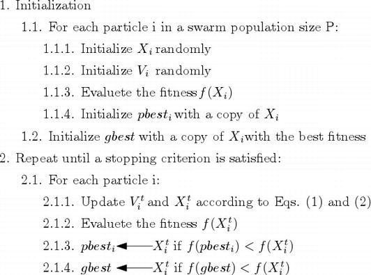
Considering a swarm with P particles, there is a position vector Xti=(xi1xi2xi3…xin)TXit=xi1xi2xi3…xinT and a velocity vector Vti=(vi1vi2vi3…vin)TVit=vi1vi2vi3…vinT at a t iteration for each one of the i particle that composes it. These vectors are updated through the dimension j according to the following equations:

Vt+1ij=wVtij+c1rt1(pbestij−Xtij)+c2rt2(gbestj−Xtij)Vijt+1=wVijt+c1r1tpbestij−Xijt+c2r2tgbestj−XijtE1

and

Xt+1ij=Xtij+Vt+1ijXijt+1=Xijt+Vijt+1

where i = 1,2,…,P and j = 1,2,…,n.

Eq. (1) denotes that there are three different contributions to a particle’s movement in an iteration, so there are three terms in it that are going to be further discussed. Meanwhile, Eq. (2) updates the particle’s positions. The parameter ww is the inertia weight constant, and for the classical PSO version, it is a positive constant value. This parameter is important for balancing the global search, also known as exploration (when higher values are set), and local search, known as exploitation (when lower values are set). In terms of this parameter, one may notice that it is one of the main differences between classical version of PSO and other versions derived from it.

Velocity update equation’s first term is a product between parameter w and particle’s previous velocity, which is the reason it denotes a particles’ previous motion into the current one. Hence, for example, if w=1w=1, the particle’s motion is fully influenced by its previous motion, so the particle may keep going in the same direction. On the other hand, if 0≤w<10≤w<1, such influence is reduced, which means that a particle rather goes to other regions in the search domain. Therefore, as the inertia weight parameter is reduced, the swarm may explore more areas in the searching domain, which means that the chances of finding a global optimum may increase. However, there is a price when using lower w values, which is the simulations turn out to be more time consuming [1].

The individual cognition term, which is the second term of Eq. (1), is calculated by means of the difference between the particle’s own best position, for example, pbestijpbestij, and its current position XtijXijt. One may notice that the idea behind this term is that as the particle gets more distant from the pbestijpbestij position, the difference (pbestij−Xtij)pbestij−Xijt must increase; therefore, this term increases, attracting the particle to its best own position. The parameter c1c1 existing as a product in this term is a positive constant and it is an individual-cognition parameter, and it weighs the importance of particle’s own previous experiences. The other parameter that composes the product of second term is r1r1, and this is a random value parameter with [0,1]01 range. This random parameter plays an important role, as it avoids premature convergences, increasing the most likely global optima [1].

Finally, the third term is the social learning one. Because of it, all particles in the swarm are able to share the information of the best point achieved regardless of which particle had found it, for example, gbestjgbestj. Its format is just like the second term, the one regarding the individual learning. Thus, the difference (gbestj−Xtij)gbestj−Xijt acts as an attraction for the particles to the best point until found at some tt iteration. Similarly, c2c2 is a social learning parameter, and it weighs the importance of the global learning of the swarm. And r2r2 plays exactly the same role as r1r1.

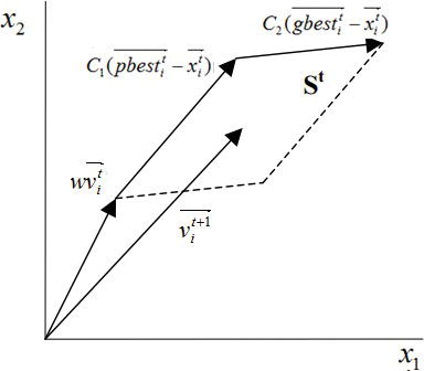
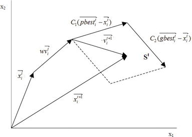
Lastly, Figure 1 shows the PSO algorithm flowchart, and one may notice that the optimization logic in it searches for minimums and all position vectors are assessed by the function f(X)fX, known as fitness function. Besides that, Figures 2 and 3 present the update in a particle’s velocity and in its position at a tt iteration, regarding a bi-dimensional problem with variables x1x1 and x2.